Glossary
Quantum computation is marked by a set of unitary matrices (quantum gates) acting on qubit states followed by measurement. The most used representation is the circuit model of computation, comprising straight lines and boxes. The horizontal lines represent qubits and boxes represent single qubit unitary gates. A two qubit unitary gate links one qubit from another via vertical lines. Some useful notations are given below.
Quantum States[edit]
- X basis/Diagonal basis/x basis:
- Z basis/Rectilinear basis/+ basis:


Unitary Operations[edit]
- Failed to parse (SVG (MathML can be enabled via browser plugin): Invalid response ("Math extension cannot connect to Restbase.") from server "https://wikimedia.org/api/rest_v1/":): {\displaystyle \text{X (NOT gate)}} :
- :


Thus, Failed to parse (SVG (MathML can be enabled via browser plugin): Invalid response ("Math extension cannot connect to Restbase.") from server "https://wikimedia.org/api/rest_v1/":): {\displaystyle |0\rangle } , Failed to parse (SVG (MathML can be enabled via browser plugin): Invalid response ("Math extension cannot connect to Restbase.") from server "https://wikimedia.org/api/rest_v1/":): {\displaystyle |1\rangle } are eigenstates of Z gate and Failed to parse (SVG (MathML can be enabled via browser plugin): Invalid response ("Math extension cannot connect to Restbase.") from server "https://wikimedia.org/api/rest_v1/":): {\displaystyle |+\rangle} , Failed to parse (SVG (MathML can be enabled via browser plugin): Invalid response ("Math extension cannot connect to Restbase.") from server "https://wikimedia.org/api/rest_v1/":): {\displaystyle |-\rangle } are eigenstates of X gate.
- Failed to parse (SVG (MathML can be enabled via browser plugin): Invalid response ("Math extension cannot connect to Restbase.") from server "https://wikimedia.org/api/rest_v1/":): {\displaystyle \text{H (Hadamard gate)}} : Failed to parse (SVG (MathML can be enabled via browser plugin): Invalid response ("Math extension cannot connect to Restbase.") from server "https://wikimedia.org/api/rest_v1/":): {\displaystyle H|0\rangle \,\to\,\ |+\rangle } or Failed to parse (SVG (MathML can be enabled via browser plugin): Invalid response ("Math extension cannot connect to Restbase.") from server "https://wikimedia.org/api/rest_v1/":): {\displaystyle H|1\rangle \,\to\,\ |-\rangle }
- Failed to parse (SVG (MathML can be enabled via browser plugin): Invalid response ("Math extension cannot connect to Restbase.") from server "https://wikimedia.org/api/rest_v1/":): {\displaystyle \text{P (Phase Gate)}} : Gates in this class operate on a single qubit. They are represented by 2 x 2 matrices of the form Failed to parse (SVG (MathML can be enabled via browser plugin): Invalid response ("Math extension cannot connect to Restbase.") from server "https://wikimedia.org/api/rest_v1/":): {\displaystyle R(\theta)} , as shown below. Here Failed to parse (SVG (MathML can be enabled via browser plugin): Invalid response ("Math extension cannot connect to Restbase.") from server "https://wikimedia.org/api/rest_v1/":): {\displaystyle \theta} is the phase shift.
Failed to parse (SVG (MathML can be enabled via browser plugin): Invalid response ("Math extension cannot connect to Restbase.") from server "https://wikimedia.org/api/rest_v1/":): {\displaystyle R(\theta)= \left[ {\begin{array}{cc} 1 & 0 \\ 0 & e^{i\theta} \\ \end{array} }\right],\quad X= \left[ {\begin{array}{cc} 0 & 1 \\ 1 & 0 \\ \end{array} }\right],\quad Z= \left[ {\begin{array}{cc} 1 & 0 \\ 0 & -1 \\ \end{array} }\right],\quad H=\frac{1}{\sqrt{2}} \left[ {\begin{array}{cc} 1 & 1 \\ 1 & -1 \\ \end{array} }\right]\quad }
- Failed to parse (SVG (MathML can be enabled via browser plugin): Invalid response ("Math extension cannot connect to Restbase.") from server "https://wikimedia.org/api/rest_v1/":): {\displaystyle \text{Controlled-U(CU)}} : uses two inputs, control qubit and target qubit. It operates U on the second(target) qubit only when the first (source) qubit is 1. C-U gates are used to produce entangled states, when the target qubit is Failed to parse (SVG (MathML can be enabled via browser plugin): Invalid response ("Math extension cannot connect to Restbase.") from server "https://wikimedia.org/api/rest_v1/":): {\displaystyle |+\rangle} and control qubit is not an eigenstate of U. In the given equation 'i' denotes the source qubit and 'j', the target qubit. Following are two important C-U gates.
Failed to parse (SVG (MathML can be enabled via browser plugin): Invalid response ("Math extension cannot connect to Restbase.") from server "https://wikimedia.org/api/rest_v1/":): {\displaystyle \text{Controlled-NOT(C-X or CNOT): }CX_{ij}|+\rangle_i|0\rangle_j\,\to\,\ \frac{1}{\sqrt{2}} (|0_i0_j\rangle+|1_i1_j\rangle)}
Failed to parse (SVG (MathML can be enabled via browser plugin): Invalid response ("Math extension cannot connect to Restbase.") from server "https://wikimedia.org/api/rest_v1/":): {\displaystyle \text{Controlled-Z (C-Z):}CZ_{ij}|+\rangle_i|+\rangle_j\,\to\,\ \frac{1}{\sqrt{2}} (|0_i+_j\rangle+|1_i-_j\rangle)}
The commutation relations for the above gates are as follows:
Failed to parse (SVG (MathML can be enabled via browser plugin): Invalid response ("Math extension cannot connect to Restbase.") from server "https://wikimedia.org/api/rest_v1/":): {\displaystyle XH=HZ,\quad XZ=-ZX}
Failed to parse (SVG (MathML can be enabled via browser plugin): Invalid response ("Math extension cannot connect to Restbase.") from server "https://wikimedia.org/api/rest_v1/":): {\displaystyle (X\otimes I)CZ=CZ(X\otimes Z),\quad(Z\otimes I)CZ=CZ(Z\otimes I)}
Hierarchy of Quantum Gates[edit]
There are different class of quantum gates as follows,
- Pauli Gates(U): Single Qubit Gates I (Identity), X, Y, Z. All the gates in this set follow Failed to parse (SVG (MathML can be enabled via browser plugin): Invalid response ("Math extension cannot connect to Restbase.") from server "https://wikimedia.org/api/rest_v1/":): {\displaystyle U^2=I}
- Clifford Gates(C): Pauli Gates, Phase Gate, C-NOT. This set of gates can be simulated on classical computer. All the gates in this set follow CU=U'C, where U and U' are two different Pauli gates depending on C
- Universal Set of gates: This set consists of all Clifford gates and one Non-Clifford gate (T gate). If a model can realise Universal Set of gates, it can imlement any quantum computation efficiently. T gates follow Failed to parse (SVG (MathML can be enabled via browser plugin): Invalid response ("Math extension cannot connect to Restbase.") from server "https://wikimedia.org/api/rest_v1/":): {\displaystyle UT=P^aU'T}
, where P is the phase gate and U, U' are any two Pauli gates depending on T. Parameter Failed to parse (SVG (MathML can be enabled via browser plugin): Invalid response ("Math extension cannot connect to Restbase.") from server "https://wikimedia.org/api/rest_v1/":): {\displaystyle a\in \{0,1\}}
is obtained from U, such that Failed to parse (SVG (MathML can be enabled via browser plugin): Invalid response ("Math extension cannot connect to Restbase.") from server "https://wikimedia.org/api/rest_v1/":): {\displaystyle P^0=I}
, Failed to parse (SVG (MathML can be enabled via browser plugin): Invalid response ("Math extension cannot connect to Restbase.") from server "https://wikimedia.org/api/rest_v1/":): {\displaystyle P^1=P}
.
To summarize, if Failed to parse (SVG (MathML can be enabled via browser plugin): Invalid response ("Math extension cannot connect to Restbase.") from server "https://wikimedia.org/api/rest_v1/":): {\displaystyle C^1=} P, Failed to parse (SVG (MathML can be enabled via browser plugin): Invalid response ("Math extension cannot connect to Restbase.") from server "https://wikimedia.org/api/rest_v1/":): {\displaystyle C^2=} C, Failed to parse (SVG (MathML can be enabled via browser plugin): Invalid response ("Math extension cannot connect to Restbase.") from server "https://wikimedia.org/api/rest_v1/":): {\displaystyle C^3=} T, then Failed to parse (SVG (MathML can be enabled via browser plugin): Invalid response ("Math extension cannot connect to Restbase.") from server "https://wikimedia.org/api/rest_v1/":): {\displaystyle C^{k}=\{U:UQU=C^{k-1}|Q\in C^1\}}
Magic States[edit]
It is any state that, if you have an unlimited supply of them, can be used to give you universal quantum computation when used in conjunction with perfect Clifford operations. The standard example is that if you can produce the state Failed to parse (SVG (MathML can be enabled via browser plugin): Invalid response ("Math extension cannot connect to Restbase.") from server "https://wikimedia.org/api/rest_v1/":): {\displaystyle (|0 \rangle +e^{i \pi/4}|1 \rangle )/ \sqrt{2}} , then you can combine this with Clifford operations in order to apply a T gate, and we know that T+Clifford is universal.
Universal Resource[edit]
A set of Failed to parse (SVG (MathML can be enabled via browser plugin): Invalid response ("Math extension cannot connect to Restbase.") from server "https://wikimedia.org/api/rest_v1/":): {\displaystyle |+_\theta\rangle } states on which applying Clifford operations is enough for universal quantum computation.
Superposition[edit]
Superposition is a fundamental concept in quantum mechanics which states if two states Failed to parse (SVG (MathML can be enabled via browser plugin): Invalid response ("Math extension cannot connect to Restbase.") from server "https://wikimedia.org/api/rest_v1/":): {\displaystyle |\psi\rangle} and Failed to parse (SVG (MathML can be enabled via browser plugin): Invalid response ("Math extension cannot connect to Restbase.") from server "https://wikimedia.org/api/rest_v1/":): {\displaystyle |\phi\rangle} are representing two valid state in a Hilbert space, their linear combination exist in the same Hilbert space as well and refer to another valid states. We call state Failed to parse (SVG (MathML can be enabled via browser plugin): Invalid response ("Math extension cannot connect to Restbase.") from server "https://wikimedia.org/api/rest_v1/":): {\displaystyle \alpha|\psi\rangle + \beta|\phi\rangle} a superposition of the two states. This property leads to most of the non-classical properties of quantum mechanics such as entanglement.
Entangled States[edit]
An entangled state is the quantum state of a group of particled (or a two party or multiparty system) that cannot be described as the independent states of these particles (or subsystems). The subsystems of such a quantum state, have quantum correlation even over a long distance. Mathematically, a multiparty entangled state cannot be written in following way:
Failed to parse (SVG (MathML can be enabled via browser plugin): Invalid response ("Math extension cannot connect to Restbase.") from server "https://wikimedia.org/api/rest_v1/":): {\displaystyle |\psi_{1-N}\rangle = |\psi_1\rangle \otimes ... \otimes |\psi_N\rangle}
The states that can be written in the above from, are called separable states.
EPR Pairs[edit]
EPR pairs refer to the pairs of particles with a conjugate physical property such as angular momentum. This concept has been introduced for the first time by the EPR (Einstein–Podolsky–Rosen) paradox which is a thought experiment challenging the explanation of physical reality provided by Quantum Mechanics.
The particles that have been used in the EPR paradox had perfect correlation in such a way that measuring a quantity of a particle A will cause the conjugated quantity of particle B to become undetermined, even if there was no contact, no classical disturbance. A two party quantum state with the above property can be described with the following state:
Failed to parse (SVG (MathML can be enabled via browser plugin): Invalid response ("Math extension cannot connect to Restbase.") from server "https://wikimedia.org/api/rest_v1/":): {\displaystyle |\Phi^+\rangle = \frac{1}{\sqrt{2}} (|00\rangle + |11\rangle)}
This is one of the Bell states.
Bell States[edit]
Bell states are maximally-entangled two-qubit states. These are the states that violate the Bell's inequality with maximal value of Failed to parse (SVG (MathML can be enabled via browser plugin): Invalid response ("Math extension cannot connect to Restbase.") from server "https://wikimedia.org/api/rest_v1/":): {\displaystyle 2\sqrt{2}}
. These states make a compelete basis for the two-qubit (4 dimensional) Hilbert space:
Failed to parse (SVG (MathML can be enabled via browser plugin): Invalid response ("Math extension cannot connect to Restbase.") from server "https://wikimedia.org/api/rest_v1/":): {\displaystyle |\Phi^{+}\rangle = \frac{1}{\sqrt{2}}(|0\rangle_{A}\otimes |0\rangle_{B}+|1\rangle_{A}\otimes |1\rangle_{B}) }
Failed to parse (SVG (MathML can be enabled via browser plugin): Invalid response ("Math extension cannot connect to Restbase.") from server "https://wikimedia.org/api/rest_v1/":): {\displaystyle |\Phi ^{-}\rangle =\frac{1}{\sqrt{2}}(|0\rangle_{A}\otimes |0\rangle_{B}-|1\rangle_{A}\otimes |1\rangle_{B}) }
Failed to parse (SVG (MathML can be enabled via browser plugin): Invalid response ("Math extension cannot connect to Restbase.") from server "https://wikimedia.org/api/rest_v1/":): {\displaystyle |\Psi ^{+}\rangle =\frac{1}{\sqrt{2}}(|0\rangle_{A}\otimes |1\rangle_{B}+|1\rangle_{A}\otimes |0\rangle_{B}) }
Bell State Measurement[edit]
Bell state measurement is termed as the projection of two qubits into one of the four Bell States as described above. It is done operating a Hadamard gate on one qubit and then, operating a C-NOT gate with this qubit as control and the other qubit as target. More on BSM can be found in [1]
Fidelity[edit]
The Fidelity is a quantum distance measure between two quantum states. For two general state $\rho$ and $\sigma$ it is defined as followes:
Failed to parse (SVG (MathML can be enabled via browser plugin): Invalid response ("Math extension cannot connect to Restbase.") from server "https://wikimedia.org/api/rest_v1/":): {\displaystyle F(\rho, \sigma) = [Tr(\sqrt{\sqrt{\rho}\sigma\sqrt{\rho}})]^2}
The definition reduces to the squared overlap between the pure states Failed to parse (SVG (MathML can be enabled via browser plugin): Invalid response ("Math extension cannot connect to Restbase.") from server "https://wikimedia.org/api/rest_v1/":): {\displaystyle |\psi_{\rho}\rangle$ and $|\psi_{\sigma}\rangle}
:
Failed to parse (SVG (MathML can be enabled via browser plugin): Invalid response ("Math extension cannot connect to Restbase.") from server "https://wikimedia.org/api/rest_v1/":): {\displaystyle F(|\psi_{\rho}\rangle, |\psi_{\sigma}\rangle) = |\langle\psi_{\rho}|\psi_{\sigma}\rangle|^2}
Density Matrix, Pure and Mixed states[edit]
A density matrix is the matrix representation of a statistical state in quantum mechanics. This is a useful representation for mixed states. The mixed states are the states which cannot be described with a single vector $|\psi\rangle$ in Hilbert space. Instead, they are statistical mixture of several pure states. These states are also useful for describing the quantum state of a subsystem of a multi-party or larger quantum sysytem where the overall state can be shown as pure states. a density matrix in general can be shown as:
Failed to parse (SVG (MathML can be enabled via browser plugin): Invalid response ("Math extension cannot connect to Restbase.") from server "https://wikimedia.org/api/rest_v1/":): {\displaystyle \rho = \sum_{i} p_i |\psi_i\rangle\langle\psi_i|}
where Failed to parse (SVG (MathML can be enabled via browser plugin): Invalid response ("Math extension cannot connect to Restbase.") from server "https://wikimedia.org/api/rest_v1/":): {\displaystyle |\psi_i\rangle}
are pure states and Failed to parse (SVG (MathML can be enabled via browser plugin): Invalid response ("Math extension cannot connect to Restbase.") from server "https://wikimedia.org/api/rest_v1/":): {\displaystyle p_i}
are the relative probabilities. For a pure quantum state Failed to parse (SVG (MathML can be enabled via browser plugin): Invalid response ("Math extension cannot connect to Restbase.") from server "https://wikimedia.org/api/rest_v1/":): {\displaystyle |\psi\rangle}
the density matrix representation will be:
Failed to parse (SVG (MathML can be enabled via browser plugin): Invalid response ("Math extension cannot connect to Restbase.") from server "https://wikimedia.org/api/rest_v1/":): {\displaystyle \rho = |\psi\rangle\langle\psi|}
Unitary transformation[edit]
A unitary transformation is an isomorphism between two Hilbert spaces, These transformation preserve the inner products of the vector states and can be shown as matrices where Failed to parse (SVG (MathML can be enabled via browser plugin): Invalid response ("Math extension cannot connect to Restbase.") from server "https://wikimedia.org/api/rest_v1/":): {\displaystyle UU^{\dagger} = U^{\dagger}U = I} .
Monogomy of entanglement[edit]
Monogamy is one of the most fundamental properties of entanglement and can, in its extremal form, be expressed as follows: If two qubits A and B are maximally quantumly correlated they cannot be correlated at all with a third qubit C. In general, there is a trade-off between the amount of entanglement between qubits A and B and the same qubit A and qubit C. This is mathematically expressed as:
Failed to parse (SVG (MathML can be enabled via browser plugin): Invalid response ("Math extension cannot connect to Restbase.") from server "https://wikimedia.org/api/rest_v1/":): {\displaystyle E(A|B1) + E(A|B2) \leq E(A|B1B2)}
where Failed to parse (SVG (MathML can be enabled via browser plugin): Invalid response ("Math extension cannot connect to Restbase.") from server "https://wikimedia.org/api/rest_v1/":): {\displaystyle E()}
is a measure for entanglement.
Ancilla or Ancillary states[edit]
Ancillary states are extra states used in some quantum algorithms and are usually measured or discarded at the end of the procedure or they represent the state of an extra quantum system that is used for computation or etc.
Bloch Sphere[edit]
In quantum mechanics, the Bloch sphere is a geometrical representation of the pure state space of a two-level quantum mechanical system (qubit). The Bloch sphere is a unit 2-sphere, with antipodal points corresponding to a pair of mutually orthogonal state vectors. The north and south poles of the Bloch sphere are typically chosen to correspond to the standard basis vectors Failed to parse (SVG (MathML can be enabled via browser plugin): Invalid response ("Math extension cannot connect to Restbase.") from server "https://wikimedia.org/api/rest_v1/":): {\displaystyle |0\rangle} , Failed to parse (SVG (MathML can be enabled via browser plugin): Invalid response ("Math extension cannot connect to Restbase.") from server "https://wikimedia.org/api/rest_v1/":): {\displaystyle |1\rangle} respectively, which in turn might correspond e.g. to the spin-up and spin-down states of an electron. This choice is arbitrary, however. The points on the surface of the sphere correspond to the pure states of the system, whereas the interior points correspond to the mixed states.
Quantum One Way Function[edit]
- Classical To Quantum QOWF
Based on the fundamental principles of quantum mechanics, QOWF was proposed by Gottesman and Chuang [2] and its definition is presented as follows.
Definition 1 Let k, Failed to parse (SVG (MathML can be enabled via browser plugin): Invalid response ("Math extension cannot connect to Restbase.") from server "https://wikimedia.org/api/rest_v1/":): {\displaystyle |f_k\rangle}
be classical bits string of length Failed to parse (SVG (MathML can be enabled via browser plugin): Invalid response ("Math extension cannot connect to Restbase.") from server "https://wikimedia.org/api/rest_v1/":): {\displaystyle L_1}
, quantum state of Failed to parse (SVG (MathML can be enabled via browser plugin): Invalid response ("Math extension cannot connect to Restbase.") from server "https://wikimedia.org/api/rest_v1/":): {\displaystyle L_2}
qubits, respectively. A function Failed to parse (SVG (MathML can be enabled via browser plugin): Invalid response ("Math extension cannot connect to Restbase.") from server "https://wikimedia.org/api/rest_v1/":): {\displaystyle f : k\rightarrow |f_k\rangle}
, where Failed to parse (SVG (MathML can be enabled via browser plugin): Invalid response ("Math extension cannot connect to Restbase.") from server "https://wikimedia.org/api/rest_v1/":): {\displaystyle |f_k\rangle}
satisfies Failed to parse (SVG (MathML can be enabled via browser plugin): Invalid response ("Math extension cannot connect to Restbase.") from server "https://wikimedia.org/api/rest_v1/":): {\displaystyle \langle f_k|f_{k'}\rangle\le\delta < 1}
for Failed to parse (SVG (MathML can be enabled via browser plugin): Invalid response ("Math extension cannot connect to Restbase.") from server "https://wikimedia.org/api/rest_v1/":): {\displaystyle k\ne k'}
, is called a QOWF under physical mechanics if
- Easy to compute: The mapping Failed to parse (SVG (MathML can be enabled via browser plugin): Invalid response ("Math extension cannot connect to Restbase.") from server "https://wikimedia.org/api/rest_v1/":): {\displaystyle f : k\rightarrow |f_k\rangle} is easy to compute by a quantum polynomial-time algorithm.
- Hard to invert: Given Failed to parse (SVG (MathML can be enabled via browser plugin): Invalid response ("Math extension cannot connect to Restbase.") from server "https://wikimedia.org/api/rest_v1/":): {\displaystyle |f_k\rangle} , it is impossible to invert k by virtue of fundamental quantum information theory.
Gate Teleportation[edit]
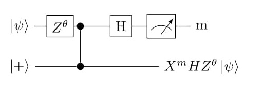
The idea comes from one-qubit teleporation. This means that one can transfer an unknown qubit |ψi without actually sending it via a quantum channel. The underlying equations explain the notion. See Figure 1 for circuit.

Failed to parse (SVG (MathML can be enabled via browser plugin): Invalid response ("Math extension cannot connect to Restbase.") from server "https://wikimedia.org/api/rest_v1/":): {\displaystyle (H\otimes I)(CZ_{12})|\psi\rangle_1|+\rangle_2}
Failed to parse (SVG (MathML can be enabled via browser plugin): Invalid response ("Math extension cannot connect to Restbase.") from server "https://wikimedia.org/api/rest_v1/":): {\displaystyle (H\otimes I)(CZ_{12})(a|0\rangle_1+b|1\rangle_1)|+\rangle_2}
Failed to parse (SVG (MathML can be enabled via browser plugin): Invalid response ("Math extension cannot connect to Restbase.") from server "https://wikimedia.org/api/rest_v1/":): {\displaystyle (H\otimes I)(a|0\rangle_1|+\rangle_2+b|1\rangle_1|-\rangle_2)}
Failed to parse (SVG (MathML can be enabled via browser plugin): Invalid response ("Math extension cannot connect to Restbase.") from server "https://wikimedia.org/api/rest_v1/":): {\displaystyle a|+\rangle_1|+\rangle_2+b|-\rangle_1|-\rangle_2}
Failed to parse (SVG (MathML can be enabled via browser plugin): Invalid response ("Math extension cannot connect to Restbase.") from server "https://wikimedia.org/api/rest_v1/":): {\displaystyle |0\rangle_1\otimes(a|+\rangle_2+b|-\rangle_2)+|1\rangle_1\otimes(a|+\rangle_2-b|-\rangle_2)}
Failed to parse (SVG (MathML can be enabled via browser plugin): Invalid response ("Math extension cannot connect to Restbase.") from server "https://wikimedia.org/api/rest_v1/":): {\displaystyle |0\rangle_1\otimes(a|+\rangle_2+b|-\rangle_2)+|1\rangle_1\otimes X(a|+\rangle_2+b|-\rangle_2)}
Failed to parse (SVG (MathML can be enabled via browser plugin): Invalid response ("Math extension cannot connect to Restbase.") from server "https://wikimedia.org/api/rest_v1/":): {\displaystyle |0\rangle_1\otimes H(a\rangle 0\rangle _2+b\rangle 1\rangle _2)+|1\rangle _1\otimes XH(a|0\rangle _2+b|1\rangle _2)}
Failed to parse (SVG (MathML can be enabled via browser plugin): Invalid response ("Math extension cannot connect to Restbase.") from server "https://wikimedia.org/api/rest_v1/":): {\displaystyle |0\rangle _1\otimes H|\psi\rangle _2+|1\rangle _1\otimes X|\psi\rangle _2}
Failed to parse (SVG (MathML can be enabled via browser plugin): Invalid response ("Math extension cannot connect to Restbase.") from server "https://wikimedia.org/api/rest_v1/":): {\displaystyle |m\rangle \otimes X^mH|\psi\rangle}
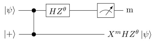
Similarly if we have the input state rotated by a Failed to parse (SVG (MathML can be enabled via browser plugin): Invalid response ("Math extension cannot connect to Restbase.") from server "https://wikimedia.org/api/rest_v1/":): {\displaystyle \mathrm{Z}(\theta)}
gate the circuit would look like Figure 2a. As the rotation gate Failed to parse (SVG (MathML can be enabled via browser plugin): Invalid response ("Math extension cannot connect to Restbase.") from server "https://wikimedia.org/api/rest_v1/":): {\displaystyle \mathrm{Z}(\theta)}
commutes with Controlled-Phase gate. Hence, Figure 2b is justified.
-
 2(a)Modified Input
 -
 2(b)Gate Teleportation


This shows that for a pair of Failed to parse (SVG (MathML can be enabled via browser plugin): Invalid response ("Math extension cannot connect to Restbase.") from server "https://wikimedia.org/api/rest_v1/":): {\displaystyle \mathrm{CZ}} entangled qubits, if the second qubit is in Failed to parse (SVG (MathML can be enabled via browser plugin): Invalid response ("Math extension cannot connect to Restbase.") from server "https://wikimedia.org/api/rest_v1/":): {\displaystyle |+\rangle} state (not an eigen value of Failed to parse (SVG (MathML can be enabled via browser plugin): Invalid response ("Math extension cannot connect to Restbase.") from server "https://wikimedia.org/api/rest_v1/":): {\displaystyle \mathrm{Z}} ) then one can teleport (transfer) the first qubit state operated by any unitary gate Failed to parse (SVG (MathML can be enabled via browser plugin): Invalid response ("Math extension cannot connect to Restbase.") from server "https://wikimedia.org/api/rest_v1/":): {\displaystyle \mathrm{U}} to the second qubit by performing operations only on the first qubit and measuring it. Next, we would need to make certain Pauli corrections (in this case Failed to parse (SVG (MathML can be enabled via browser plugin): Invalid response ("Math extension cannot connect to Restbase.") from server "https://wikimedia.org/api/rest_v1/":): {\displaystyle {\mathrm{X}}^{\mathrm{m}}} ) to obtain Failed to parse (SVG (MathML can be enabled via browser plugin): Invalid response ("Math extension cannot connect to Restbase.") from server "https://wikimedia.org/api/rest_v1/":): {\displaystyle \mathrm{U}|\psi\rangle} . In other words, we can say the operated state is teleported to the second qubit by a rotated basis measurement of the first qubit with additional Pauli corrections.
Graph states[edit]
The above operation can also be viewed as a graph state with two nodes and one edge. The qubit 1 is measured in a rotated basis Failed to parse (SVG (MathML can be enabled via browser plugin): Invalid response ("Math extension cannot connect to Restbase.") from server "https://wikimedia.org/api/rest_v1/":): {\displaystyle \mathrm{HZ}(\theta)}
, thus leaving qubit 2 in desired state and Pauli Correction Failed to parse (SVG (MathML can be enabled via browser plugin): Invalid response ("Math extension cannot connect to Restbase.") from server "https://wikimedia.org/api/rest_v1/":): {\displaystyle \mathrm{X}^|\mathrm{s1}\rangle \mathrm{HZ}(\theta_1)|\psi\rangle}
, where Failed to parse (SVG (MathML can be enabled via browser plugin): Invalid response ("Math extension cannot connect to Restbase.") from server "https://wikimedia.org/api/rest_v1/":): {\displaystyle \mathrm{s1}}
is the measurement outcome of qubit 1. See Figure 3

Now, suppose we need to operate the state with two unitary gates Failed to parse (SVG (MathML can be enabled via browser plugin): Invalid response ("Math extension cannot connect to Restbase.") from server "https://wikimedia.org/api/rest_v1/":): {\displaystyle \mathrm{Z}(\theta_1)}
and Failed to parse (SVG (MathML can be enabled via browser plugin): Invalid response ("Math extension cannot connect to Restbase.") from server "https://wikimedia.org/api/rest_v1/":): {\displaystyle \mathrm{Z}(\theta_2)}
. This can be done by taking the output state of Failed to parse (SVG (MathML can be enabled via browser plugin): Invalid response ("Math extension cannot connect to Restbase.") from server "https://wikimedia.org/api/rest_v1/":): {\displaystyle \mathrm{Z}(\theta_1)}
gate as the input state of Failed to parse (SVG (MathML can be enabled via browser plugin): Invalid response ("Math extension cannot connect to Restbase.") from server "https://wikimedia.org/api/rest_v1/":): {\displaystyle \mathrm{Z}(\theta_2)}
gate and then repeating gate teleportation for this setup, as described above. Thus, following the same pattern for graph states we have now three nodes (two measurement qubits for two operators and one output qubit) with two edges, entangled as one dimensional chain (See Figure 4).

The measurement on qubit Failed to parse (SVG (MathML can be enabled via browser plugin): Invalid response ("Math extension cannot connect to Restbase.") from server "https://wikimedia.org/api/rest_v1/":): {\displaystyle \mathrm{1}} will operate Failed to parse (SVG (MathML can be enabled via browser plugin): Invalid response ("Math extension cannot connect to Restbase.") from server "https://wikimedia.org/api/rest_v1/":): {\displaystyle \mathrm{X}^{\mathrm{s1}}\mathrm{HZ}(\theta_1)|\psi\rangle\otimes I} on qubits Failed to parse (SVG (MathML can be enabled via browser plugin): Invalid response ("Math extension cannot connect to Restbase.") from server "https://wikimedia.org/api/rest_v1/":): {\displaystyle \mathrm{2}} and Failed to parse (SVG (MathML can be enabled via browser plugin): Invalid response ("Math extension cannot connect to Restbase.") from server "https://wikimedia.org/api/rest_v1/":): {\displaystyle \mathrm{3}} . If qubit Failed to parse (SVG (MathML can be enabled via browser plugin): Invalid response ("Math extension cannot connect to Restbase.") from server "https://wikimedia.org/api/rest_v1/":): {\displaystyle \mathrm{2}} when measured in the given basis yields outcome Failed to parse (SVG (MathML can be enabled via browser plugin): Invalid response ("Math extension cannot connect to Restbase.") from server "https://wikimedia.org/api/rest_v1/":): {\displaystyle \mathrm{s2}} , qubit Failed to parse (SVG (MathML can be enabled via browser plugin): Invalid response ("Math extension cannot connect to Restbase.") from server "https://wikimedia.org/api/rest_v1/":): {\displaystyle \mathrm{3}} results in the following state Failed to parse (SVG (MathML can be enabled via browser plugin): Invalid response ("Math extension cannot connect to Restbase.") from server "https://wikimedia.org/api/rest_v1/":): {\displaystyle {\mathrm{X}}^{\mathrm{s2}}\mathrm{HZ}(\theta_2){\mathrm{X}}^{\mathrm{s1}}\mathrm{HZ}(\theta_1)|\psi\rangle} . Using the relation we shift all the Pauli corrections to one end i.e. qubit Failed to parse (SVG (MathML can be enabled via browser plugin): Invalid response ("Math extension cannot connect to Restbase.") from server "https://wikimedia.org/api/rest_v1/":): {\displaystyle \mathrm{3}} becomes Failed to parse (SVG (MathML can be enabled via browser plugin): Invalid response ("Math extension cannot connect to Restbase.") from server "https://wikimedia.org/api/rest_v1/":): {\displaystyle {\mathrm{X}}^{\mathrm{s2}}\mathrm{HZ}(\theta_2)\mathrm{HZ}(\theta_1)|\psi\rangle} (Failed to parse (SVG (MathML can be enabled via browser plugin): Invalid response ("Math extension cannot connect to Restbase.") from server "https://wikimedia.org/api/rest_v1/":): {\displaystyle {\mathrm{Z}}^{\mathrm{s1}}\mathrm{H}={\mathrm{HX}}^{\mathrm{s1}}} ). This method of computation requires sequential measurement of states i.e. all the states should not be measured simultaneously. As outcome of qubit Failed to parse (SVG (MathML can be enabled via browser plugin): Invalid response ("Math extension cannot connect to Restbase.") from server "https://wikimedia.org/api/rest_v1/":): {\displaystyle \mathrm{1}} can be used to choose sign of Failed to parse (SVG (MathML can be enabled via browser plugin): Invalid response ("Math extension cannot connect to Restbase.") from server "https://wikimedia.org/api/rest_v1/":): {\displaystyle \pm\theta_2} . This technique is also known as adaptive measurement. With each measurement, the qubits before the one measured at present have been destroyed by measurement. It is a feed-forward mechanism, hence known as one way quantum computation.
Measurement Based Quantum Computation (MBQC)[edit]
MBQC is a formalism used for quantum computation by operating only single qubit measurements on a fixed set of entangled states, also known as graph states. Graph states denote any graph where each node represents a quantum state, and the edges denote entanglement between any two vertices. The measurement on successive layers of qubits is decided by previous measurement outcomes. Outcomes of last qubit layer gives the result of concerned computation. Following, we illustrate certain primitives necessary to understand the working of MBQC.
Cluster States[edit]
In case of multi-qubit quatum circuits, one needs a 2-dimensional graph state. Cluster State is a square lattice used as substrate for such computation. All the nodes are in Failed to parse (SVG (MathML can be enabled via browser plugin): Invalid response ("Math extension cannot connect to Restbase.") from server "https://wikimedia.org/api/rest_v1/":): {\displaystyle |+\rangle}
entangled by Failed to parse (SVG (MathML can be enabled via browser plugin): Invalid response ("Math extension cannot connect to Restbase.") from server "https://wikimedia.org/api/rest_v1/":): {\displaystyle \mathrm{CZ}}
indicated by the edges. It is known to be universal i.e. it can simulate any quatum gate.

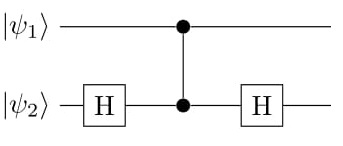
Each row would thus represent the teleporation of starting qubit in that row horizontally. On the other hand, vertical edges indicate different input qubits linked with multi-qubit gates (same as circuit model). For example, see Figure Figure 6 to understand the conversion from circuit model to graph state model. As the computation relation follows Failed to parse (SVG (MathML can be enabled via browser plugin): Invalid response ("Math extension cannot connect to Restbase.") from server "https://wikimedia.org/api/rest_v1/":): {\displaystyle X=HZH}
, thus, Figure Figure 6a represents Circuit diagram for Failed to parse (SVG (MathML can be enabled via browser plugin): Invalid response ("Math extension cannot connect to Restbase.") from server "https://wikimedia.org/api/rest_v1/":): {\displaystyle \mathrm{CNOT}}
gate in terms of Failed to parse (SVG (MathML can be enabled via browser plugin): Invalid response ("Math extension cannot connect to Restbase.") from server "https://wikimedia.org/api/rest_v1/":): {\displaystyle \mathrm{CZ}}
gate and Single Qubit Gate Failed to parse (SVG (MathML can be enabled via browser plugin): Invalid response ("Math extension cannot connect to Restbase.") from server "https://wikimedia.org/api/rest_v1/":): {\displaystyle \mathrm{H}}
.
-
 (a)Circuit Diagram to implement C-NOT
 -
 (b)Graph State Pattern for C-NOT


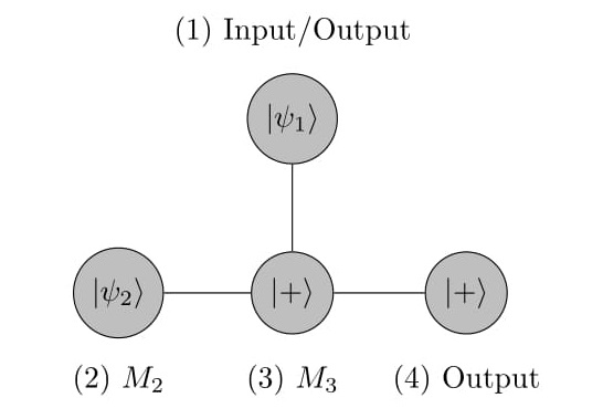
Figure 6b shows implementation of the first Hadamard gate on the second input state as measurement Failed to parse (SVG (MathML can be enabled via browser plugin): Invalid response ("Math extension cannot connect to Restbase.") from server "https://wikimedia.org/api/rest_v1/":): {\displaystyle \mathrm{M}_\mathrm{2}}
on qubit Failed to parse (SVG (MathML can be enabled via browser plugin): Invalid response ("Math extension cannot connect to Restbase.") from server "https://wikimedia.org/api/rest_v1/":): {\displaystyle \mathrm{2}}
. Then Failed to parse (SVG (MathML can be enabled via browser plugin): Invalid response ("Math extension cannot connect to Restbase.") from server "https://wikimedia.org/api/rest_v1/":): {\displaystyle \mathrm{CZ}}
gate is implemented by the entangled qubits Failed to parse (SVG (MathML can be enabled via browser plugin): Invalid response ("Math extension cannot connect to Restbase.") from server "https://wikimedia.org/api/rest_v1/":): {\displaystyle \mathrm{3}}
and Failed to parse (SVG (MathML can be enabled via browser plugin): Invalid response ("Math extension cannot connect to Restbase.") from server "https://wikimedia.org/api/rest_v1/":): {\displaystyle \mathrm{1}}
in the graph state. Qubit Failed to parse (SVG (MathML can be enabled via browser plugin): Invalid response ("Math extension cannot connect to Restbase.") from server "https://wikimedia.org/api/rest_v1/":): {\displaystyle \mathrm{3}}
is entangled to another qubit Failed to parse (SVG (MathML can be enabled via browser plugin): Invalid response ("Math extension cannot connect to Restbase.") from server "https://wikimedia.org/api/rest_v1/":): {\displaystyle \mathrm{4}}
to record the output while measurement Failed to parse (SVG (MathML can be enabled via browser plugin): Invalid response ("Math extension cannot connect to Restbase.") from server "https://wikimedia.org/api/rest_v1/":): {\displaystyle \mathrm{M}_\mathrm{3}}
on qubit Failed to parse (SVG (MathML can be enabled via browser plugin): Invalid response ("Math extension cannot connect to Restbase.") from server "https://wikimedia.org/api/rest_v1/":): {\displaystyle \mathrm{3}}
implements the second Hadamard gate. Finally, the states to which qubits Failed to parse (SVG (MathML can be enabled via browser plugin): Invalid response ("Math extension cannot connect to Restbase.") from server "https://wikimedia.org/api/rest_v1/":): {\displaystyle \mathrm{(1)}}
and Failed to parse (SVG (MathML can be enabled via browser plugin): Invalid response ("Math extension cannot connect to Restbase.") from server "https://wikimedia.org/api/rest_v1/":): {\displaystyle \mathrm{(4)}}
are reduced to determine the output states of the two input qubits after Failed to parse (SVG (MathML can be enabled via browser plugin): Invalid response ("Math extension cannot connect to Restbase.") from server "https://wikimedia.org/api/rest_v1/":): {\displaystyle \mathrm{CNOT}}
gate operation.
It is evident that one needs to remove certain nodes from the cluster state in order to implement the above shown graph state. This can be done by Z-basis measurements. Such measurements would leave the remaining qubits in the cluster state with extra Pauli corrections. This can be explained as follows. Consider a two-dimesional graph state Failed to parse (SVG (MathML can be enabled via browser plugin): Invalid response ("Math extension cannot connect to Restbase.") from server "https://wikimedia.org/api/rest_v1/":): {\displaystyle \{\mathrm{1,2}\}}
. If qubit Failed to parse (SVG (MathML can be enabled via browser plugin): Invalid response ("Math extension cannot connect to Restbase.") from server "https://wikimedia.org/api/rest_v1/":): {\displaystyle \mathrm{1}}
is to be eliminated, we operate Failed to parse (SVG (MathML can be enabled via browser plugin): Invalid response ("Math extension cannot connect to Restbase.") from server "https://wikimedia.org/api/rest_v1/":): {\displaystyle \mathrm{CZ}}
with Failed to parse (SVG (MathML can be enabled via browser plugin): Invalid response ("Math extension cannot connect to Restbase.") from server "https://wikimedia.org/api/rest_v1/":): {\displaystyle \mathrm{2}}
as target and Failed to parse (SVG (MathML can be enabled via browser plugin): Invalid response ("Math extension cannot connect to Restbase.") from server "https://wikimedia.org/api/rest_v1/":): {\displaystyle \mathrm{1}}
as control.
Failed to parse (SVG (MathML can be enabled via browser plugin): Invalid response ("Math extension cannot connect to Restbase.") from server "https://wikimedia.org/api/rest_v1/":): {\displaystyle {\mathrm{CZ}}_{\mathrm{12}}{|+\rangle}_{1}|+\rangle_2=|0\rangle_1|+\rangle_2+|1\rangle_1|-\rangle_2}
Thus, if measurement on Failed to parse (SVG (MathML can be enabled via browser plugin): Invalid response ("Math extension cannot connect to Restbase.") from server "https://wikimedia.org/api/rest_v1/":): {\displaystyle \mathrm{1}}
yields Failed to parse (SVG (MathML can be enabled via browser plugin): Invalid response ("Math extension cannot connect to Restbase.") from server "https://wikimedia.org/api/rest_v1/":): {\displaystyle \mathrm{m}}
, qubit Failed to parse (SVG (MathML can be enabled via browser plugin): Invalid response ("Math extension cannot connect to Restbase.") from server "https://wikimedia.org/api/rest_v1/":): {\displaystyle \mathrm{2}}
would be in the state Failed to parse (SVG (MathML can be enabled via browser plugin): Invalid response ("Math extension cannot connect to Restbase.") from server "https://wikimedia.org/api/rest_v1/":): {\displaystyle \mathrm{Z}^\mathrm{m}|+\rangle}
. Hence, such Z-basis measurements invoke an extra Failed to parse (SVG (MathML can be enabled via browser plugin): Invalid response ("Math extension cannot connect to Restbase.") from server "https://wikimedia.org/api/rest_v1/":): {\displaystyle \mathrm{Z}^\mathrm{m}}
Pauli correction on all the neighbouring sites of 1 with 1 eliminated, in the resulting graph state.
Thus, to summarise, we design a measurement pattern from gate teleportation circuit of the desired computation as shown above. The cluster state is converted into the required graph state by Z-basis measurement on extraneous sites. Measuring all the qubits in the required basis and we get the required computation in the form of classical outcome register from measurement of the last layer of qubits. If it is a quantum function, the last layer of qubits is the output quantum register.
Brickwork States[edit]
Although cluster states are universal for MBQC, yet we need to tailor these to the specific computation by performing some computational (Z) basis measurements. If we were to use this principle for blind quantum computing, Client would have to reveal information about the structure of the underlying graph state. Thus, for the UBQC protocol, we introduce a new family of states called the Brickwork states which are universal for X − Y plane measurements and thus do not require the initial computational basis measurements. It was later shown that the Z-basis measurements can be dropped for cluster states and hence cluster states are also universal in X-Y measurements.

Definition 1 A brickwork state Gn×m, where m ≡ 5 (mod 8), is an entangled state of n × m qubits constructed as follows (see also Figure 7):
- Prepare all qubits in state |+i and assign to each qubit an index (i,j), i being a column (i ∈ [n]) and j being a row (j ∈ [m]).
- For each row, apply the operator c-Z on qubits (i,j) and (i,j + 1) where 1 ≤ j ≤ m − 1.
- For each column j ≡ 3 (mod 8) and each odd row i, apply the operator c-Z on qubits (i,j) and (i + 1,j) and also on qubits (i,j + 2) and (i + 1,j + 2).
- For each column j ≡ 7 (mod 8) and each even row i, apply the operator c-Z on qubits (i,j) and (i + 1,j) and also on qubits (i,j + 2) and (i + 1,j + 2).
Cylinder Brickwork States[edit]
The cylinder brickwork state Failed to parse (SVG (MathML can be enabled via browser plugin): Invalid response ("Math extension cannot connect to Restbase.") from server "https://wikimedia.org/api/rest_v1/":): {\displaystyle G^{C}_{n*m}} is a modification of the brickwork state of size Failed to parse (SVG (MathML can be enabled via browser plugin): Invalid response ("Math extension cannot connect to Restbase.") from server "https://wikimedia.org/api/rest_v1/":): {\displaystyle n*m} , for even n, where the first and the last rows are connected such that the regular brickwork structure is preserved while introducing rotational symmetry. A tape Failed to parse (SVG (MathML can be enabled via browser plugin): Invalid response ("Math extension cannot connect to Restbase.") from server "https://wikimedia.org/api/rest_v1/":): {\displaystyle T_i} , shown in Fig 8.3, present in a cylinder brickwork graph is the subgraph which includes all the states in the random rows Failed to parse (SVG (MathML can be enabled via browser plugin): Invalid response ("Math extension cannot connect to Restbase.") from server "https://wikimedia.org/api/rest_v1/":): {\displaystyle i} and Failed to parse (SVG (MathML can be enabled via browser plugin): Invalid response ("Math extension cannot connect to Restbase.") from server "https://wikimedia.org/api/rest_v1/":): {\displaystyle i + 1} .
If all the nodes in Failed to parse (SVG (MathML can be enabled via browser plugin): Invalid response ("Math extension cannot connect to Restbase.") from server "https://wikimedia.org/api/rest_v1/":): {\displaystyle T_i} of the graph Failed to parse (SVG (MathML can be enabled via browser plugin): Invalid response ("Math extension cannot connect to Restbase.") from server "https://wikimedia.org/api/rest_v1/":): {\displaystyle G^{C}_{n*m}} are prepared in the dummy qubit state, Failed to parse (SVG (MathML can be enabled via browser plugin): Invalid response ("Math extension cannot connect to Restbase.") from server "https://wikimedia.org/api/rest_v1/":): {\displaystyle |z\rangle} where Failed to parse (SVG (MathML can be enabled via browser plugin): Invalid response ("Math extension cannot connect to Restbase.") from server "https://wikimedia.org/api/rest_v1/":): {\displaystyle z \in {0,1}} and the rest of the nodes are prepared in the state Failed to parse (SVG (MathML can be enabled via browser plugin): Invalid response ("Math extension cannot connect to Restbase.") from server "https://wikimedia.org/api/rest_v1/":): {\displaystyle |+_{\theta_i}\rangle} , then after entangling according to the cylinder brickwork state, the nodes are completely disentangled from the rest of the graph. The final obtained graph would be Failed to parse (SVG (MathML can be enabled via browser plugin): Invalid response ("Math extension cannot connect to Restbase.") from server "https://wikimedia.org/api/rest_v1/":): {\displaystyle G^{C}_{(n-1)*m} \bigotimes^{m}_{i=1} |z\rangle} .
The steps to perform single trap verifiable universal blind quantum computing are:
- A random qubit is chosen to be the trap qubit (red node in Fig 8.1)
- All other vertices in the tape containing the trap qubit (solid black nodes in Fig 8.2), are set to be dummy qubits
- This results in an isolated trap qubit in the state Failed to parse (SVG (MathML can be enabled via browser plugin): Invalid response ("Math extension cannot connect to Restbase.") from server "https://wikimedia.org/api/rest_v1/":): {\displaystyle |+_{\theta_i}\rangle} together with many dummy qubits after entanglement operations (Fig 8.3)
- The net result, after discarding the dummy qubits, is a disentangled trap qubit in a product state with a brickwork state (Fig 8.4)
Flow Construction-Determinism[edit]
Measurement outcomes of qubits is not certain, hence it renders MBQC a non-deterministic model. This can still be rectified by invoking Pauli corrections based on the previous outcomes, as evident from above. For example, to implement Hadamard gate on input state Failed to parse (SVG (MathML can be enabled via browser plugin): Invalid response ("Math extension cannot connect to Restbase.") from server "https://wikimedia.org/api/rest_v1/":): {\displaystyle |\psi\rangle = a|0\rangle + b|1\rangle}
, we consider the case of a two qubit graph state Failed to parse (SVG (MathML can be enabled via browser plugin): Invalid response ("Math extension cannot connect to Restbase.") from server "https://wikimedia.org/api/rest_v1/":): {\displaystyle \mathcal{C}_{2\text{x}1}}
.
If one measures qubit i in Failed to parse (SVG (MathML can be enabled via browser plugin): Invalid response ("Math extension cannot connect to Restbase.") from server "https://wikimedia.org/api/rest_v1/":): {\displaystyle \{|+\rangle,|-\rangle\}}
basis and gets outcome s, qubit j reduces to,
Failed to parse (SVG (MathML can be enabled via browser plugin): Invalid response ("Math extension cannot connect to Restbase.") from server "https://wikimedia.org/api/rest_v1/":): {\displaystyle =(a-b)|0\rangle+(a+b)|1\rangle, \text{if s=1}}
As, the two possible output states are different, it shows this method is non-deterministic. One could end up with any of the two states and there is no certainty. Nevertheless, we observe that if X gate is operated on the second qubit after measurement if outcome is 1, both the equations would be same and hence, obtained state is Failed to parse (SVG (MathML can be enabled via browser plugin): Invalid response ("Math extension cannot connect to Restbase.") from server "https://wikimedia.org/api/rest_v1/":): {\displaystyle H|\psi\rangle}
.
Flow construction is the semanticism to construct the measurement pattern for a given graph state. It gives the Pauli corrections for a particular qubit in the graph state, called X and Z dependencies. In simpler words, it records the effect of shifting all Pauli X and Z corrections to the left of (after performing) Entanglement and Entanglement operations, respectively, for each qubit. The result is recorded as sets of X, Z corrections required for each site. These sets depend on the graph state and not the computation or measurement results. Hence, it can be computed while choosing the graph state for a required computation. Following we illustrate how to construct such models with ease using Measurement Calculus to invoke determinism in One-Way Quantum Computation(MBQC).
Choose a unitary gate for the circuit and hence, its measurement pattern. In order to implement this pattern on a graph state, there are four basic steps: Preparation, Entanglement, Measurement, Corrections.
- Preparation prepares all input qubits in the required state, generally represented as Failed to parse (SVG (MathML can be enabled via browser plugin): Invalid response ("Math extension cannot connect to Restbase.") from server "https://wikimedia.org/api/rest_v1/":): {\displaystyle |+_\theta=\frac{1}{\sqrt{2}}(|0\rangle+e^{i\theta}|1\rangle)} where Failed to parse (SVG (MathML can be enabled via browser plugin): Invalid response ("Math extension cannot connect to Restbase.") from server "https://wikimedia.org/api/rest_v1/":): {\displaystyle \theta\epsilon[0,2\pi]} .
- Entanglement entangles all the qubits according to the required graph state. This operation is denoted by Failed to parse (SVG (MathML can be enabled via browser plugin): Invalid response ("Math extension cannot connect to Restbase.") from server "https://wikimedia.org/api/rest_v1/":): {\displaystyle E_{ij}}
, where C-Z is operated with i as control qubit and j as target qubit.
- Measurement assigns measurement angle in X-Y plane for each qubit. Measurement operator is notated as Failed to parse (SVG (MathML can be enabled via browser plugin): Invalid response ("Math extension cannot connect to Restbase.") from server "https://wikimedia.org/api/rest_v1/":): {\displaystyle M^\alpha_i}
: the qubit ’i’ would be measured in Failed to parse (SVG (MathML can be enabled via browser plugin): Invalid response ("Math extension cannot connect to Restbase.") from server "https://wikimedia.org/api/rest_v1/":): {\displaystyle \{|+_\alpha\rangle,|-_\alpha\rangle\}}
basis i.e. if the state is Failed to parse (SVG (MathML can be enabled via browser plugin): Invalid response ("Math extension cannot connect to Restbase.") from server "https://wikimedia.org/api/rest_v1/":): {\displaystyle \frac{1}{\sqrt{2}}(|0\rangle+e^{i\alpha}|1\rangle)}
one gets outcome 0 and if the state is Failed to parse (SVG (MathML can be enabled via browser plugin): Invalid response ("Math extension cannot connect to Restbase.") from server "https://wikimedia.org/api/rest_v1/":): {\displaystyle \frac{1}{\sqrt{2}}(|0\rangle-e^{i\alpha}|1\rangle)}
, the outcome is 1.
- Correction calculates all Pauli corrections to be applied on a given qubit in the pattern. The set of such parameters are called Dependencies for X and Z operators individually. To calculate all the Pauli Corrections on a given qubit, one needs to take into account the measurement outcomes of previous qubits as well as commutation relations. Both affect the Pauli corrections for a given qubit. Below is a formalism to explain the process with an example.
The effect of X gate on a measurement angle (Failed to parse (SVG (MathML can be enabled via browser plugin): Invalid response ("Math extension cannot connect to Restbase.") from server "https://wikimedia.org/api/rest_v1/":): {\displaystyle \alpha}
) in X-Y plane is to change its sign and Z gate is to add a phase Failed to parse (SVG (MathML can be enabled via browser plugin): Invalid response ("Math extension cannot connect to Restbase.") from server "https://wikimedia.org/api/rest_v1/":): {\displaystyle \pi}
.
We shall denote measurement in X-basis (Failed to parse (SVG (MathML can be enabled via browser plugin): Invalid response ("Math extension cannot connect to Restbase.") from server "https://wikimedia.org/api/rest_v1/":): {\displaystyle M_i^0}
) as Failed to parse (SVG (MathML can be enabled via browser plugin): Invalid response ("Math extension cannot connect to Restbase.") from server "https://wikimedia.org/api/rest_v1/":): {\displaystyle M_i^x}
and Y-basis (Failed to parse (SVG (MathML can be enabled via browser plugin): Invalid response ("Math extension cannot connect to Restbase.") from server "https://wikimedia.org/api/rest_v1/":): {\displaystyle M_i^\frac{\pi}{2}}
) as Failed to parse (SVG (MathML can be enabled via browser plugin): Invalid response ("Math extension cannot connect to Restbase.") from server "https://wikimedia.org/api/rest_v1/":): {\displaystyle M_i^y}
Commutation relations:
Failed to parse (SVG (MathML can be enabled via browser plugin): Invalid response ("Math extension cannot connect to Restbase.") from server "https://wikimedia.org/api/rest_v1/":): {\displaystyle E_{ij}X_i^s=X_i^sZ_i^sE_{ij}\quad\quad (EX)}
Failed to parse (SVG (MathML can be enabled via browser plugin): Invalid response ("Math extension cannot connect to Restbase.") from server "https://wikimedia.org/api/rest_v1/":): {\displaystyle E_{ij}X_j^s=X_j^sZ_j^sE_{ij}\quad\quad(EX)}
Failed to parse (SVG (MathML can be enabled via browser plugin): Invalid response ("Math extension cannot connect to Restbase.") from server "https://wikimedia.org/api/rest_v1/":): {\displaystyle E_{ij}Z_i^t=Z_i^tE_{ij}\quad\quad(EZ)}
Failed to parse (SVG (MathML can be enabled via browser plugin): Invalid response ("Math extension cannot connect to Restbase.") from server "https://wikimedia.org/api/rest_v1/":): {\displaystyle E_{ij}Z_j^t=Z_j^tE_{ij}\quad\quad(EZ)}
Failed to parse (SVG (MathML can be enabled via browser plugin): Invalid response ("Math extension cannot connect to Restbase.") from server "https://wikimedia.org/api/rest_v1/":): {\displaystyle ^t[M^\alpha_i]^sX^r_i=^t[M^\alpha_i]^{s+r}\quad\quad(MX)}
Failed to parse (SVG (MathML can be enabled via browser plugin): Invalid response ("Math extension cannot connect to Restbase.") from server "https://wikimedia.org/api/rest_v1/":): {\displaystyle M_i^xX_i^s=M_i^x\quad\quad(MX)}
The last second equation is implied from the fact that for Failed to parse (SVG (MathML can be enabled via browser plugin): Invalid response ("Math extension cannot connect to Restbase.") from server "https://wikimedia.org/api/rest_v1/":): {\displaystyle M_i^x}
, Failed to parse (SVG (MathML can be enabled via browser plugin): Invalid response ("Math extension cannot connect to Restbase.") from server "https://wikimedia.org/api/rest_v1/":): {\displaystyle x=0=-0}
. Thus, X gate has no effect on measurement in X-basis for the given states. Using above notations we express the equation for circuit model of C-NOT from Figure 6 with two inputs and two outputs: Qubits: 1,2,3,4
Outcomes: Failed to parse (SVG (MathML can be enabled via browser plugin): Invalid response ("Math extension cannot connect to Restbase.") from server "https://wikimedia.org/api/rest_v1/":): {\displaystyle s_1, s_2, s_3, s_4}
Circuit Operation: Failed to parse (SVG (MathML can be enabled via browser plugin): Invalid response ("Math extension cannot connect to Restbase.") from server "https://wikimedia.org/api/rest_v1/":): {\displaystyle X^{s_3}_4M_3^xE_{34}E_{13}X_3^{s_2}M_2^xE_{23}}
Failed to parse (SVG (MathML can be enabled via browser plugin): Invalid response ("Math extension cannot connect to Restbase.") from server "https://wikimedia.org/api/rest_v1/":): {\displaystyle X^{s_3}_4M_3^xE_{34}\mathbf{E_{13}X_3^{s_2}}M_2^xE_{23}\overset{\text{EX}}{\implies}}
Failed to parse (SVG (MathML can be enabled via browser plugin): Invalid response ("Math extension cannot connect to Restbase.") from server "https://wikimedia.org/api/rest_v1/":): {\displaystyle X^{s_3}_4Z_1^{s_2}M_3^x\mathbf{E_{34}X_3^{s_2}}M_2^xE_{13}E_{23}\overset{\text{EX}}{\implies}}
Failed to parse (SVG (MathML can be enabled via browser plugin): Invalid response ("Math extension cannot connect to Restbase.") from server "https://wikimedia.org/api/rest_v1/":): {\displaystyle X^{s_3}_4Z_4^{s_2}Z_1^{s_2}\mathbf{M_3^xX_3^{s_2}}M_2^xE_{13}E_{23}E_{34}\overset{\text{MX}}{\implies}}
Hence, we obtain a measurement pattern to implement C-NOT gate with a T-shaped graph state with three qubits entangled chain Failed to parse (SVG (MathML can be enabled via browser plugin): Invalid response ("Math extension cannot connect to Restbase.") from server "https://wikimedia.org/api/rest_v1/":): {\displaystyle \{2,3,4\}}
and 1 entangled to 3. X dependency sets for qubit Failed to parse (SVG (MathML can be enabled via browser plugin): Invalid response ("Math extension cannot connect to Restbase.") from server "https://wikimedia.org/api/rest_v1/":): {\displaystyle 1:\{s_3\}}
, Failed to parse (SVG (MathML can be enabled via browser plugin): Invalid response ("Math extension cannot connect to Restbase.") from server "https://wikimedia.org/api/rest_v1/":): {\displaystyle 2:\phi}
, Failed to parse (SVG (MathML can be enabled via browser plugin): Invalid response ("Math extension cannot connect to Restbase.") from server "https://wikimedia.org/api/rest_v1/":): {\displaystyle 3:\phi}
, Failed to parse (SVG (MathML can be enabled via browser plugin): Invalid response ("Math extension cannot connect to Restbase.") from server "https://wikimedia.org/api/rest_v1/":): {\displaystyle 4:\phi}
. Z dependency sets for qubit Failed to parse (SVG (MathML can be enabled via browser plugin): Invalid response ("Math extension cannot connect to Restbase.") from server "https://wikimedia.org/api/rest_v1/":): {\displaystyle 1:\{s_2\}}
, Failed to parse (SVG (MathML can be enabled via browser plugin): Invalid response ("Math extension cannot connect to Restbase.") from server "https://wikimedia.org/api/rest_v1/":): {\displaystyle 2:\phi}
, Failed to parse (SVG (MathML can be enabled via browser plugin): Invalid response ("Math extension cannot connect to Restbase.") from server "https://wikimedia.org/api/rest_v1/":): {\displaystyle 3:\phi}
, Failed to parse (SVG (MathML can be enabled via browser plugin): Invalid response ("Math extension cannot connect to Restbase.") from server "https://wikimedia.org/api/rest_v1/":): {\displaystyle 4:\{s_2\}}
. The measurements are independent of any outcome so they can all be performed in parallel. In the end, Pauli corrections are performed as such. Parity (modulo 2 sum) of all the previous outcomes in the dependency set is calculated for each qubit (i), for X (Failed to parse (SVG (MathML can be enabled via browser plugin): Invalid response ("Math extension cannot connect to Restbase.") from server "https://wikimedia.org/api/rest_v1/":): {\displaystyle s^X_i=s_1\oplus s_2\oplus...}
) and Z (Failed to parse (SVG (MathML can be enabled via browser plugin): Invalid response ("Math extension cannot connect to Restbase.") from server "https://wikimedia.org/api/rest_v1/":): {\displaystyle s^Z_i=s_1\oplus s_2\oplus...}
), separately. Thus, Failed to parse (SVG (MathML can be enabled via browser plugin): Invalid response ("Math extension cannot connect to Restbase.") from server "https://wikimedia.org/api/rest_v1/":): {\displaystyle X^{s^X_i}Z^{s^Z_i}}
is operated on qubit i.
Quantum SWAP test[edit]

Quantum SWAP test (1) helps to compare two quantum states Failed to parse (SVG (MathML can be enabled via browser plugin): Invalid response ("Math extension cannot connect to Restbase.") from server "https://wikimedia.org/api/rest_v1/":): {\displaystyle |\psi\rangle} and Failed to parse (SVG (MathML can be enabled via browser plugin): Invalid response ("Math extension cannot connect to Restbase.") from server "https://wikimedia.org/api/rest_v1/":): {\displaystyle |\psi'\rangle} . An ancilla qubit is prepared here in the state Failed to parse (SVG (MathML can be enabled via browser plugin): Invalid response ("Math extension cannot connect to Restbase.") from server "https://wikimedia.org/api/rest_v1/":): {\displaystyle \frac{|0\rangle + |1\rangle}{2}} and a controlled swap test is performed on two states Failed to parse (SVG (MathML can be enabled via browser plugin): Invalid response ("Math extension cannot connect to Restbase.") from server "https://wikimedia.org/api/rest_v1/":): {\displaystyle |\psi\rangle} and Failed to parse (SVG (MathML can be enabled via browser plugin): Invalid response ("Math extension cannot connect to Restbase.") from server "https://wikimedia.org/api/rest_v1/":): {\displaystyle |\psi'\rangle} .
If Failed to parse (SVG (MathML can be enabled via browser plugin): Invalid response ("Math extension cannot connect to Restbase.") from server "https://wikimedia.org/api/rest_v1/":): {\displaystyle |\psi\rangle} = Failed to parse (SVG (MathML can be enabled via browser plugin): Invalid response ("Math extension cannot connect to Restbase.") from server "https://wikimedia.org/api/rest_v1/":): {\displaystyle |\psi'\rangle} , then the ancilla qubit, after performing a Hadamard operation, yields Failed to parse (SVG (MathML can be enabled via browser plugin): Invalid response ("Math extension cannot connect to Restbase.") from server "https://wikimedia.org/api/rest_v1/":): {\displaystyle |0\rangle} when measurement is applied in computational basis. The SWAP test passes here.
If Failed to parse (SVG (MathML can be enabled via browser plugin): Invalid response ("Math extension cannot connect to Restbase.") from server "https://wikimedia.org/api/rest_v1/":): {\displaystyle |\psi\langle|\psi'\rangle \leq \delta} , then the ancilla qubit, after performing a Hadamard Gate and upon measurement, passes the test with probability Failed to parse (SVG (MathML can be enabled via browser plugin): Invalid response ("Math extension cannot connect to Restbase.") from server "https://wikimedia.org/api/rest_v1/":): {\displaystyle \frac{1+\delta^2}{2}} and fails the test with probability Failed to parse (SVG (MathML can be enabled via browser plugin): Invalid response ("Math extension cannot connect to Restbase.") from server "https://wikimedia.org/api/rest_v1/":): {\displaystyle \frac{1-\delta^2}{2}} . Hence, the SWAP test always passes for the same inputs and sometimes fails if they are different. By repeating the SWAP test, its efficiency can be amplified.
Quantum Capable Homomorphic Encryption[edit]
- Homomorphic Encryption
A homomorphic encryption scheme HE is a scheme to carry out classical computation from the Server while hiding the inputs, outputs and computation. It can be divided into following four stages. - Key Generation. The algorithm (pk,evk,sk) ← HE.Keygen(1λ) takes a λ, a security parameter as input and outputs a public key encryption key pk, a public evaluation key evk and a secret decryption key sk.
- Encryption. The algorithm c ← HE.Encpk(µ) takes the public key pk and a single bit message µ ∈ {0,1} and outputs a ciphertext c. The notation HE.Encpk(µ;r) is be used to represent the encryption of a bit µ using randomness r.
- Decryption. The algorithm µ∗ ← HE.Decsk(c) takes the secret key sk and a ciphertext c and outputs a message µ∗ ∈ {0,1}.
- Homomorphic Evaluation The algorithm cf ← HE.Evalevk(f,c1,...,cl) takes the evaluation key evk, a function f : {0,1}l → {0,1} and a set of l ciphertexts c1,...,cl, and outputs a ciphertext cf. It must be the case that:
HE.Decsk(cf) = f(HE.Decsk(c1),...,HE.Decsk(cl)) (1) with all but negligible probability in λ. This means classical HE decrypts ciphertext bit by bit. HE scheme is compact if HE.Eval is independent of any inputs or computation. It is fully homomorphic if it can compute any boolean computation.
- Quantum Capable: A classical HE scheme is quantum capable if it can be used to evaluate quantum circuits. Any HE scheme to be quantum capable requires the following two properties.
- invariance of ciphertext:
- natural XOR operation: